Table of Contents
Python Imports
from IPython.display import Image
from IPython.core.display import HTML
import pickle

#Import Plotting Libraries
import matplotlib.pyplot as plt
import seaborn as sns
from yellowbrick.regressor import ResidualsPlot

#Importing Dependencies
import pandas as pd
import numpy as np
from numpy import nan
import ast
import requests
from urllib.parse import urljoin, urlunsplit, urlparse
import bs4
from bs4 import BeautifulSoup
from bs4.element import Comment

from collections import Counter
from string import punctuation
import csv

import newspaper
from newspaper import Article
from newspaper import fulltext

# Tokenization Of Sentences
import nltk
# nltk.download('punkt')

#Readability Scores
import textstat
from sklearn.linear_model import LinearRegression, ElasticNetCV, RidgeCV, LassoCV
from sklearn.metrics import mean_squared_error
from sklearn.model_selection import train_test_split, cross_val_score, cross_val_predict
from sklearn.preprocessing import StandardScaler

# GridSearch
from sklearn.model_selection import GridSearchCV

# Scipy Integration for Sparse Matrixes
from scipy import sparse

# Additional Feature Engineering - NLP Text Data Import
from sklearn.feature_extraction.text import TfidfVectorizer
cleaned_df = pd.read_pickle('Pickled_Data_Files/final_df.pkl')
Executive Summary
The primary aim was to predict the number of shares an article would earn after being published on the internet for 1 year.
The selected topics were:
- Affiliate Marketing
- Content Marketing
- Copy-writing
- Display Advertising
- Email Marketing
- Growth Hacking
- Influencer Marketing
- Link Building
- Marketing Automation
- Performance Marketing
- Podcast Marketing
- Search Engine Marketing
- Social Media Marketing
- Video Marketing
- Website Design
Evaluation Metrics
The evaluation metrics were MeanSquaredError (MSE) and the mean $R^2$ score from 5 cross validated train-test splits of either the standalone models or grid searched bestestimators.
Error Function: Minimizing The Residual Sum of Squares is the error function which will be used to evaluate the regression models.
Using a variety of regression models, the best predictive score was 0.85 $R^2$ from 100 random forest regressor estimators as an ensemble method.
Taking the logarithm + 1 - $log(y)+1$ of the target variable ('Total Shares') improved the model's $R^2$ score from 0.35 $R^2$ to 0.85 $R^2$.
The most important coefficients that impact the shareability of an article are:
- Evergreen Score (0 - 100)
- Does the article have article amplifiers? (True / False)
- Does The Article Page Have Referring Domains (True / False)
Negative coefficients that decreased the chance of an article being shared are:
- Number of Linking Pages
- SSL Encryption (True / False)
- Meta Description Length
The predictive power that we have gained is only applicable to models that are 1 year or older as this is where our sampling was applied.
Audience
Content creation is a time consuming and valuable activity. The time that marketers spend producing content must be classified as a treasured resource and needs to be effectively optimized.
Audience - Digital marketers: who wish to understand what are the key factors/variables that can make an article more shareable than another.
- Discovering what are the core components of a successful article will empower and help marketers to create more impactful and shareable content.
Objective
To predict the number of shares an article will accumulate after 1 year. This allows us to avoid the additional bias as some articles accumulate a large amount of shares quickly after being published due to the news cycle.
The predictive features used are:
- Technical On-Page Metrics (Page Load Speed, No SSL/SSL etc).
- On-Page Word Metrics (Word Count, Unique Word Count, Number of Sentences).
- Unique, Impactful Words via TF-IDF Vectorization (Every word is counted and assigned a score via the TF-IDF algorithim).
- Link Metrics: The number of backlinks pointing to the HTML page.
- Buzzsumo Metrics: Evergreen Score + Article Amplifiers.
The Process
1. Data Collection
- 30,000 Article URL's were collected via the BuzzSumo's Pro Plan.
- 15 topics were selected within the digital marketing niche to see if the topic of an article could influence it's shareability.
- A custom web crawler was created that allowed for the extraction of 61 metrics including the article text, HTML content.
- Google's Page Speed API was utilised to extract page speed metrics for every article.
2. Pre-processing
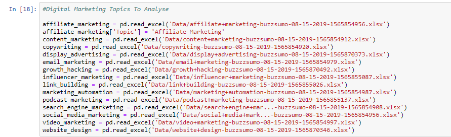
Firstly 15 topics were downloaded from BuzzSumo's pro plan, these topics were selected by performing keyword research in Ahrefs , the keywords with the highest monthly search volume were chosen to be topics.
Every row within each spreadsheet was labelled with it's appropriate topic.
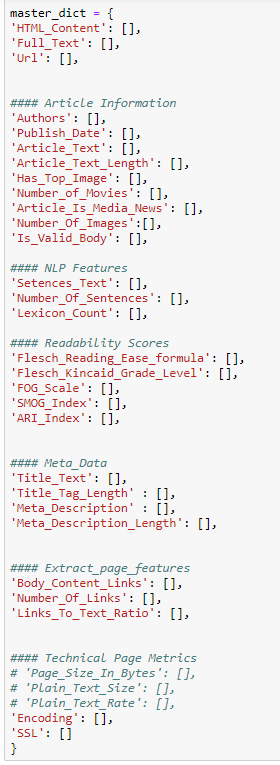
Firstly I created a data structure for the Python Web Crawler to capture a range of features from the HTML web page. This included article information, NLP features, readability scores, meta data and technical features such as whether the web page was secure or not (HTTPS vs HTTP).
Cleaning The BuzzSumo Data
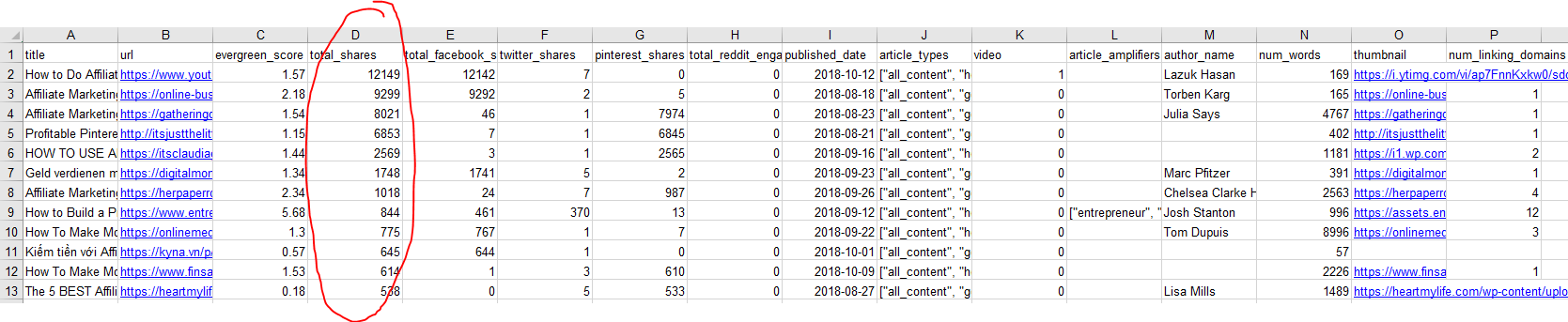
Our target variable is defined as the total_shares in column D, also there were additional columns that I decided to drop such as:
- Thumbnail
- Video
- twitter_shares, pinterest_shares, total_reddit_engagement (These metrics are directly correlated with our target variable and therefore we cannot use them within our machine learning models)
Dummifying Variables
Additionally I decided to 'dummify' the non-numerical columns so that these variables could be used for predictive modeling.
You can see an example of creating dummy variables below based on the different article types:

Merging Datasets (BuzzSumo + Web Scraped Data)
Then both of these datasets were merged enabling us to not only use BuzzSumo's metrics for prediction, but also any useful features from the web crawled articles.
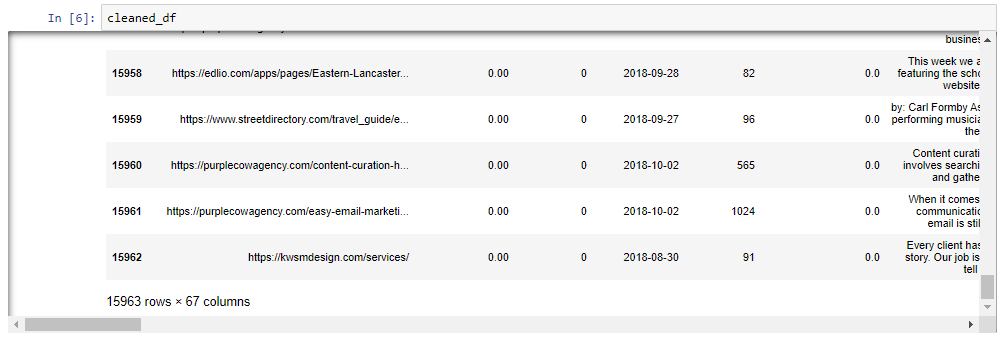
The combined dataset size was 15,963 articles with 67 features.
Merging Datasets (Cleaned DataFrame + WebPageSpeed Data From Google Page Speed Insights API)
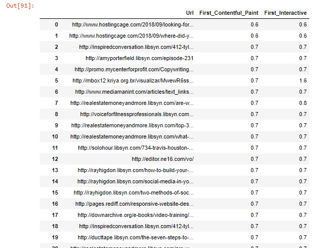
During a 1 week period the Google Page Speed Insights API was queried for 1 week. The web page speed data was obtained for 14469/15743 URL's. Again the two datasets were merged by the URL as the foreign key for both dataframes.
3. EDA - Exploratory Data Analysis
cleaned_df
cleaned_df.info()
cleaned_df.describe()
cleaned_df.corr()[['Total_Shares']].sort_values(by='Total_Shares', ascending=False)[1:].head(12)
cleaned_df.corr()[['Total_Shares']].sort_values(by='Total_Shares', ascending=False).tail(12)
fig, ax = plt.subplots(figsize=(12,6))
sns.distplot(cleaned_df['Total_Shares'], color='purple', bins=90)
plt.title('The Distribution Of Article Shares', pad=30, fontsize='21')
plt.xlabel('Number of Article Shares', fontsize='16', labelpad=20)
plt.ylabel('Counts',  fontsize='16', labelpad=20)
plt.savefig('Article_Share_Distribution',dpi=200)
plt.show()

As you can see in the above graph our target variable is highly skewed and is not normally distributed. This means that majority of articles only receive a small number of shares.
Additionally the target variable is more likely to be from an exponential distribution.
Article Data EDA - Distributions For Positively Correlated Predictor Variables In Relation To The Target Variable
fig, (ax1, ax2,  ax3, ax4) = plt.subplots(figsize=(20, 6), ncols=4)
sns.distplot(cleaned_df['Evergreen_Score'].sort_values(ascending=False), ax = ax1)
sns.distplot(cleaned_df['Word_Count'].sort_values(ascending=False), ax = ax2)
sns.distplot(cleaned_df['num_linking_domains'].sort_values(ascending=False), ax = ax3)
sns.distplot(cleaned_df['Number_Of_Sentences'].sort_values(ascending=False), ax = ax4)
plt.savefig('X_Predictor_Variables_1',dpi=200)
plt.show()

fig, (ax1, ax2,  ax3, ax4) = plt.subplots(figsize=(20, 6), ncols=4)

sns.distplot(cleaned_df['Lexicon_Count'].sort_values(ascending=False), ax = ax1)
sns.distplot(cleaned_df['Plain_Text_Size'].sort_values(ascending=False), ax = ax2)
sns.distplot(cleaned_df['Article_Text_Length'].sort_values(ascending=False), ax = ax3)
sns.distplot(cleaned_df['Has_Author_Name'].sort_values(ascending=False), ax = ax4)
plt.savefig('X_Predictor_Variables_2',dpi=200)

plt.show()

Article Types EDA - What Article Type Is Shared Mostly Frequently?
article_types = [(x, cleaned_df.groupby(x)) for x in cleaned_df.columns if x.startswith('article')]
article_data = [(item[0], item[1].Total_Shares.mean().values) for item in article_types]
article_types = [(x, cleaned_df.groupby(x)) for x in cleaned_df.columns if x.startswith('article')]
fig, ax = plt.subplots(figsize=(12,12))
article_data = [(item[0], item[1].Total_Shares.mean().values[-1]) for item in article_types]
article_data.sort(key= lambda x: x[1])
plt.barh([item[0] for item in article_data], width = [item[1] for item in article_data] )
plt.xticks(rotation = 90)
plt.xlabel('Mean Shares - μ ', fontsize='16', labelpad=20)
plt.ylabel('Article Types',  fontsize='16', labelpad=20)
plt.title('Articles Grouped By Type Of Content', pad=30, fontsize='21')
plt.tight_layout()
plt.savefig('Article_Types',dpi=200)
plt.show()

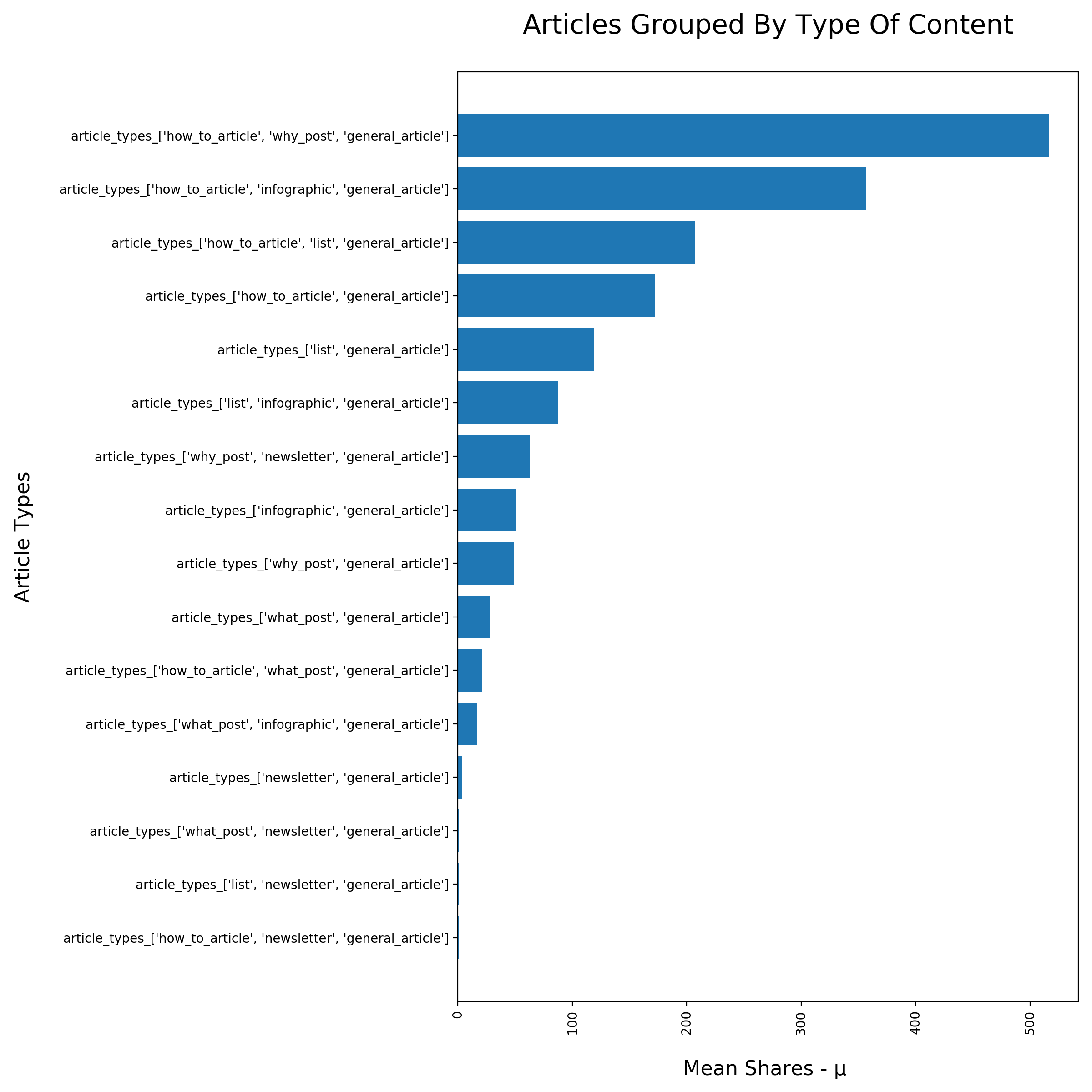
Articles that are tagged "how to articles" & "why post" on average received the most amount of shares, this was followed by infographics and list articles.
Therefore the insight that we can gain from this is that people reading digital marketing topics actively share content that is more educational (how to), visual (infographic) and easily digestible (list articles).
Topic Type EDA - What Topic Is Shared Mostly Frequently?
group_by_objects = []

for x in cleaned_df.columns:
    if x.startswith('Topic_'):
        group_by_objects.append((x , cleaned_df.groupby(x)))
topic_data = [(item[0], item[1].Total_Shares.mean().values[1]) for item in group_by_objects]
topic_data.sort(key= lambda x: x[1])
fig, ax = plt.subplots(figsize=(12,12))
plt.bar([item[0] for item in topic_data], height = [item[1] for item in topic_data])
plt.xticks(rotation = 45)
plt.xlabel('Topics', fontsize='16', labelpad=20)
plt.ylabel('Mean Shares - μ',  fontsize='16', labelpad=20)
plt.title('Articles Grouped By Topic - What Topic Is Shared Mostly Frequently?', pad=30, fontsize='21')
plt.tight_layout()
plt.savefig('Article_Topic_Types',dpi=200)
plt.show()

Search Engine Marketing was the most shared topic and was closely followed by Growth Marketing & Social Media Marketing.
The mean shares was considerably lower for topics such as website design and display advertising. Hence carefully selecting topics that are shared more on average could be a useful way to:
- Earn more backlinks, social mentions and publicity.
4. Model Selection + Evaluation
As we will be using TF-IDF, the matrices are often sparse in shape and large in terms of dimensionality (~3,000 columns by 15,000 rows).
Therefore a custom pipeline and grid search was created, allowing for optimization of:
- The Model hyperparameters
- The TFID pre-processing stage
The following models were trialled:
- Linear Regression
- Ridge (Linear Regression)
- Lasso (Linear Regression)
- Decision Tree Regressor
- RandomForest Regressor (100 RandomForest Models)
- ADA GradientBoostingRegressor with a RandomForest Ensemble
5. Results / Findings
df = pickle.load(open('Pickled_Data_Files/results.pkl', 'rb')).reset_index(drop=True)
df
df.iloc[:, [0,1, 2,3, 4, 6]]
The most impactful model utilised a logged + 1 target variable, with 5 bagged forest random regressor's serving as the base estimator for the AdaBoostRegressor model.
Additionally by adding the web page speed data from Google Page Speed Insights, the mean cross validation score increased on our best model by ~ 5%.
NLP Text Data
Text data parsed through a TFID vectorizer resulted in poorer model performance for both linear regression and decision tree regressors, therefore it was excluded from the future modeling experiments.
- This is likely due to over-fitting on noisy text data
- Also random forests struggle to use all of the correct features as the matrix increases in dimensional size and sparsity.
Linear Regression
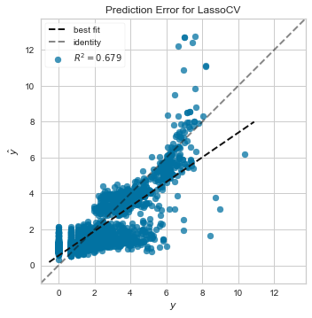
The linear regression model with non-logged data produced better scores than our baseline, however the mean cross validation scores were negative. This suggested that there was multi-collinearity inside of the data, which was reduced after applying regularization via the Lasso + Ridge regression models.
lasso_residuals = pickle.load(open('Pickled_Data_Files/lasso_residuals.pkl', 'rb'))
# Residual Plot
fig, ax = plt.subplots(figsize=(20,9))
sns.distplot(lasso_residuals)
plt.xlabel('', fontsize='16', labelpad=20)
plt.title('The Distribution Of Residuals From A LassoCV Model', pad=30, fontsize='25')
plt.savefig('Residuals_Distribution',dpi=200)
plt.show()

After taking the logarithm of the target variable, applying LassoCV we can see that the shape of the residuals is normally distributed. This means we can reliably make inference from the coefficient values (linear regression models rely on the assumption that the residuals are normally distributed).
## Lasso Coeficients ###
lasso_coefficients = pickle.load(open('Pickled_Data_Files/lasso_coefficients.pkl', 'rb'))
lasso_coefficients.columns = ['Coefficients']

fig, ax = plt.subplots(figsize=(20,9))
x_values =  lasso_coefficients.sort_values(by='Coefficients', ascending=False).head(10).index
sns.barplot(x=x_values, y='Coefficients',
            data=lasso_coefficients.sort_values(by='Coefficients', ascending=False).head(10))
plt.xticks(rotation = 25)
label = ax.set_title('The Top 10 Positive Coefficients From A LassoCV Model', fontsize = 24, pad=30)
plt.savefig('Positive_Coefficients_Lasso_Model',dpi=200)
plt.show()

fig, ax = plt.subplots(figsize=(20,9))
x_values =  lasso_coefficients.sort_values(by='Coefficients', ascending=True).head(10).index
sns.barplot(x=x_values, y='Coefficients',
            data=lasso_coefficients.sort_values(by='Coefficients', ascending=True).head(10))
label = ax.set_title('The Top 10 Negative Coefficients From A LassoCV Model', fontsize = 24, pad=30)
plt.xticks(rotation = 25)
plt.savefig('Negative_Coefficients_Lasso_Model',dpi=200)
plt.show()

lasso_coefficients.abs().sort_values(by='Coefficients', ascending=False).head(15)
All of the coefficients above contain:
- A logged target (y) variable.
- All variables have been stadardized with Z scores.
Therefore the current interpretation is:
- For every 1 increase/decrease of a specific X variable there is a 1 standard deviation increase/decrease which will result in an increase/decrease of log(y).
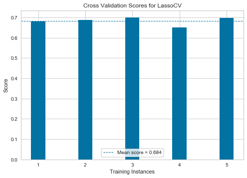
Linear Prediction Plot + Cross Validation Training Scores
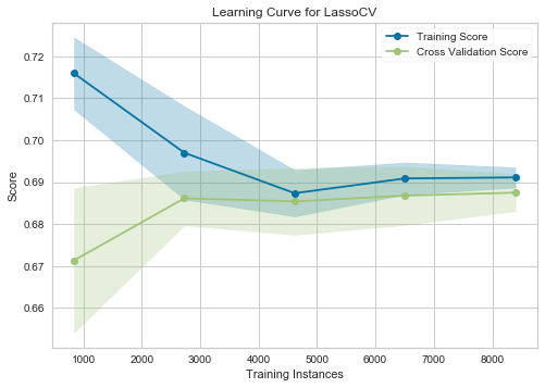
The learning curve shows us how many training observations we need to reduce the variability/standard deviation of the mean training score and the cross validation score.
After ~ 4500 observations the training score and cross validation score start to converge which shows us that we only need ~ 4500 observations to start making stable predictions.
Linear Prediction Plot + Cross Validation Training Scores

Linear Prediction Plot + Cross Validation Training Scores
Linear Prediction Plot + Cross Validation Training Scores
Logging The Target Variable + Decision Tree Regressor
As the target variable 'Total Shares' distribution looked skewed and exponential, I decided to apply a log + 1 transform to the target variable. This combined with 5 ADA boosted bagged random forest regressors (100 estimators) led to a mean cross validated training score of 0.856 $R^2$.
Decision Tree - Max Depth: 5 To View The Tree Structure

The primary features that are driving the decisions of a max_depth 5 decision tree regressor are:
- Evergreen Score
- Has Article Amplifiers
Additionally for articles that had more than 0.5 article amplifiers and a higher evergreen score than 0.155:
- 5852/12594 samples were divided by the Title_Tag_Length and an example of this can be seen below.

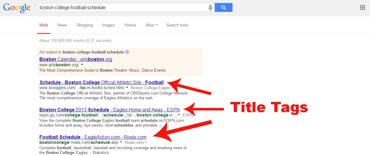
We can infer from this that having a title_tag_length > 79.5 characters causes an article to become less shareable and also if the title_tag_length is less than 45.5 the article is also less likely to be shared.
This makes sense because we want a catchy, strong headline that entices someone to click and read the article, however if the article headline is too long then it will cause the title to be truncated within the Google SERPS (search engine reuslts pages) which often leads to a lower click through rate for the article.
An example of a truncuated <'title'> tag can be seen below:

Decision Tree Regressor Feature Importances
feature_importance_values = df.iloc[5:,:]['Coefficients/Feature_Importances'].values[0]['feature_importance_values']
indexes = df.iloc[5:,:]['Coefficients/Feature_Importances'].values[0]['indexes']
feature_importance_values
feature_importances = list(zip(indexes, feature_importance_values))
new_list = sorted(feature_importances, key=lambda x: x[1], reverse= True)
fig, ax = plt.subplots(figsize=(20, 9))
sns.barplot(x = [item[1] for item in new_list]  , y = [item[0] for item in new_list])
plt.xlabel('Importance of Feature', fontsize='16', labelpad=20)
plt.ylabel('Types of Feature Importances',  fontsize='16', labelpad=20)
label = ax.set_title('The Feature Importances From A Decision Tree Regressor - Max Depth 5', fontsize = 24, pad=30)
plt.savefig('Feature_Importances_Decision_Tree_Regressor',dpi=200)
plt.show()

- Evergreen_Score: If an article is deemed to be evergreen it is meant to be non-seasonal and information that is repeatedly searched for.
- Has_Article_Amplifiers: An article amplifier is defined as a key influencer who has an audience which is largest enough to amplify the publisher's article.
Challenges
- 30,000 articles were downloaded, however I was only able to obtain the article text data for 15,000 URL's, this was due to NewsPaper3k only being able to extract the main content for $1/2$ of the article data.
- Working with text data naturally creates sparse matrices, this can be problematic because it drastically increases the dimensionality of the feature space. In order to combat this challenge, a custom standard_scaler and TFID_vectorizer class were created in sci-kit learn for optimising the pipelines and grid_search process.
- The target variable 'Total Shares' was not normally distributed and was exponentially distributed. By applying the logarithm and adding +1 to all of the values, the model captured a more linear relationship between our predictor features and our target variable.
- Some of the articles had 404'ing pages, therefore whilst web scraping excessive exception handling was required to ensure that all of the features gathered were aligned to the correct URL.
- The variables which were our best predictors are only available via BuzzSumo which means that our predictions are currently partially dependent on a 3rd party tool/data.
Risks
- The sample chosen was 1 year old, this was selected to remove any bias of an article not being online enough to receive a significant part of it's online shares. However this type of sample could lead to omission bias within the model's predictions.
- Therefore it would be advisable to study the natural share cycle of article's and the share velocity from when an article is originally published until it reaches a certain level of maturity.
Assumptions
- We have assumed that by taking 1 month's worth of content for 15 topics that our sample is representative of the population for every individual topic.
- Taking a sample of articles for a 3 month snapshot might not be a representative sample, furthermore seasonality might have an influential factor on how article's are shared across different topics.
Key Takeaways
- Focus on producing more evergreen content.
- Prioritise creating how to guides over infographics and list posts.
- Leverage relationships with key influencers to increase the number of article shares.
- Focus on producing long-form content because it was a positive coefficient within the LassoCV model (higher number of sentences).
Next Steps
- Sentiment analysis: could be performed on all of the articles as this could be influencing the shareability of an article.
- Scrape additional topics and to expand the number of article's crawled to 100,000 + articles.
- Implementing a neural network: , from having to apply a logarithm to the target variable we can clearly see that the relationship between the predictor matrix and the target variable is not linear. A neural network might be able to model effectively the non-linear relationships within our dataset.
- To scrape additional link metrics from 3rd party providers including:
- Ahrefs
- SEMrush
- Majestic
- Time Series Analysis: It would also be good idea to track articles / topics for several months or years. This would allow us to perform time series analysis on individual topics. We would then be ble to see what topics are increasing or decreasing over time and would be able to make predictions on what the number of article shares a particular topic group would receive in the future.
- Testing New Python Packages: Also it would be worth testing different scraping / article parsing libraries because NewsPaper3K was only able to scrape 50-55% of the original set of URL's. If we could improve the reliability of scraping the main content, then we would be able to acquire more data.